What You Will Learn
This post demonstrates how to achieve a 3.2x speedup in PyTorch training by systematically identifying and eliminating performance bottlenecks. We’ll start by using NVIDIA Nsight Systems to profile a typical training loop, uncovering inefficiencies such as unnecessary CPU-GPU synchronization and slow data transfers. Guided by the profiler, we’ll apply targeted fixes, like asynchronous data movement and smarter loss accumulation, that directly address the observed issues.
After resolving profiler-identified bottlenecks, we’ll layer on a series of generic PyTorch optimizations: enabling cuDNN benchmarking, compiling the model with torch.compile, using mixed precision (torch.autocast), and switching to channels-last memory format. Each step brings incremental gains, culminating in a training loop that runs over three times faster than the original baseline.
Whether you’re new to profiling or looking to maximize your hardware’s potential, this guide provides practical, real-world examples of how to combine Nsight-driven insights with best-practice PyTorch tweaks for maximum training throughput.
Meet Nsight: Your Bottleneck Detective
NVIDIA Nsight Systems is a comprehensive system-wide performance analysis tool designed to help developers optimize applications running on both CPUs and GPUs. With Nsight Systems, you can visualize the interactions between your code, the operating system, and hardware resources, making it easier to identify bottlenecks and inefficiencies.
Key capabilities include:
- Timeline visualization of CPU and GPU activity, showing how work is scheduled and executed.
- Detailed profiling of kernel launches, memory transfers, and synchronization events.
- Integration with frameworks like PyTorch and TensorFlow for deep learning workloads.
- Support for annotating code with NVTX markers to highlight specific regions of interest.
- Multi-platform support, including Linux and Windows, and compatibility with both local and remote profiling.
To install Nsight Systems follow the official NVIDIA documentation. The documentation provides a full overview of the tool’s features, supported platforms, and usage examples.
In this post, we’ll focus on using Nsight Systems to profile PyTorch training, but the same principles apply to other GPU-accelerated workloads.
Starting Baseline: The Naive Training Loop
Throughout this post, we’ll use a ResNet50 model trained on the CIFAR-10 dataset. However, the techniques and insights discussed are broadly applicable, they do not rely on this specific architecture or even on image data (with one minor exception noted later).
To keep things focused, we’ll begin with a minimal training loop. Features like checkpointing, early stopping, gradient clipping, and validation are omitted for clarity:
for epoch in range(epochs):
    model.train()
    total_loss = 0.0
    total_correct = 0
    total_samples = 0

    for inputs, targets in train_loader:
        inputs, targets = inputs.to(device), targets.to(device)

        outputs = model(inputs)
        loss = criterion(outputs, targets)
        loss.backward()
        optimizer.step()
        optimizer.zero_grad()

        total_loss += loss.item()
        preds = outputs.argmax(dim=1)
        total_correct += (preds == targets).sum().item()
        total_samples += targets.size(0)

    avg_train_loss = total_loss / len(train_loader)
    train_accuracy = total_correct / total_samples
    print(f"Epoch {(epoch+1):>3} | Train Loss: {avg_train_loss:.4f} | Acc: {train_accuracy:.4f}")
We’ll use “images per second” as our primary metric for training speed. Here’s the baseline performance before any optimizations:
[Benchmark] 994.59 images/sec
Profiling in Action: First Look with Nsight
We run Nsight with basic settings:
nsys profile --delay 10 --duration 10 python train.py
--delay 10: Waits 10 seconds before starting the profiling session, allowing initial model and data loading (and warmup) to complete. This ensures the profiler captures only the steady-state training phase.--duration 10: Specifies that profiling should run for 10 seconds, usually enough to capture steady-state behavior without generating excessively large report files.
This generates a .nsys-rep file viewable in Nsight’s visualizer.
While Nsight Systems provides a graphical interface, the typical workflow for deep learning is to run training and profiling on a remote or headless server. You use the command-line profiler to generate a .nsys-rep report file during training, then transfer this file to your local machine and open it in the Nsight visualizer for detailed analysis. This approach allows you to profile large-scale jobs without needing a display or GUI on the training server.
Here’s what the profiler output looks like in our case.
Click the image below to zoom in, examining the details is crucial!

When you open the report, you’ll see a timeline of CUDA activity with repeating forward-backward iterations. Focus on the CUDA HW row, which summarizes GPU utilization. Notice the periodic gaps, these are moments when the GPU is idle, which is a red flag.
To investigate further, zoom into a one-second segment of the 10-second trace (right-click and select “zoom into selection”). Here’s what you’ll see:

On the CUDA HW row, you’ll notice regular gaps, periods where the GPU is idle. Ideally, the GPU should be busy throughout training. Any idle time means lost performance and warrants investigation.
If you examine the timeline, you’ll notice these idle gaps consistently align with each iteration of the forward-backward training loop. Rather than simply assuming the cause, let’s see how we can add more detailed information to the profiler output. This will help us directly connect specific code sections to the observed behavior, making it easier to pinpoint exactly where and why these gaps occur.
Deep Dive: Annotating and Sampling Your Training Loop
We add more flags to the profiler:
nsys profile --delay 10 --duration 10 \
  --pytorch=autograd-shapes-nvtx \
  --python-sampling=true --backtrace=none \
  python train.py
--python-sampling=true --backtrace=none: Periodically samples the Python call stack during profiling, letting you see exactly what the CPU is doing at each moment. This is invaluable for identifying CPU-side bottlenecks.--pytorch=autograd-shapes-nvtx: Automatically adds NVTX annotations around PyTorch operations, including autograd shapes. These markers appear in the Nsight timeline, making it much easier to correlate specific PyTorch ops with GPU activity.
You can enhance your profiling by adding NVTX annotations directly in your code. These annotations create visual markers in the Nsight timeline, making it much easier to correlate code regions with GPU activity and identify bottlenecks.
For example, to highlight the forward pass in your training loop:
with torch.cuda.nvtx.range("forward"):
    outputs = model(inputs)
You can use similar annotations around other key sections (like loss calculation or backward pass) to gain deeper insight into where time is spent during training.
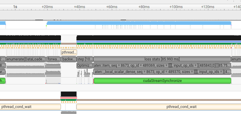
Here’s the result:

- The timeline now clearly shows the different phases: forward, backward, optimizer step, and loss stats.
- Surprisingly, the “loss stats” section takes a significant amount of CPU time.
- You’ll also notice a block labeled
enumerate(DataLoader), which aligns exactly with the periods where the GPU is idle.
Another important detail: the fourth row from the top contains orange markers. Hovering over them in Nsight reveals the Python call stack at the moment of sampling. For example:

This lets you see the full call stack in Python during specific parts of the training loop.
So, there are two main issues to investigate:
- Why does “loss stats” take so long? It’s not even an important part of the actual training.
- Why does the GPU go idle during the enumeration of the DataLoader?
Hidden Syncs: The Cost of .item()
Let’s examine the Python call stack in the “loss stats” region.

You can see that the same line is executed repeatedly throughout this region.
Line 196 in the training code, in our case, is:
total_loss += loss.item()
In Nsight, this corresponds to a call to cudaStreamSynchronize, which blocks the CPU until the GPU finishes all prior work. Since loss is on GPU and total_loss is a CPU float, calling .item() forces sync.
Notice the green marker on the CUDA API row, which perfectly aligns with the “loss stats” region, this is where a call to cudaStreamSynchronize occurs. This function is a red flag: it tells the CPU to pause and wait until all previous GPU operations are finished.
What’s happening here?
The call to loss.item() triggers this synchronization. But why does it require CPU-GPU sync, and why does it slow down training?
Since we’re training on the GPU, all tensors, including loss, reside in GPU memory. However, total_loss is a regular Python float on the CPU. To accumulate the loss, we need to transfer the value from the GPU to the CPU, which is what loss.item() does. This operation forces the CPU to wait until the GPU has finished computing the loss, causing a synchronization point via cudaStreamSynchronize. Only after this wait does the actual memory transfer from GPU to CPU occur.
Why does this hurt performance?
The main issue isn’t the CPU waiting for the GPU, nor the memory transfer itself. The real problem is that, once this synchronization happens, the GPU’s task queue is empty, the CPU stopped submitting new work while waiting. As a result, the GPU sits idle until new tasks arrive, leading to wasted compute cycles.
The solution
if a synchronization is triggered for a non-critical operation, it’s better to do it asynchronously so the CPU can keep queuing up work for the GPU. In our case, the fix is simple:
total_loss += loss.detach()
Using detach() ensures that total_loss doesn’t immediately fetch the value from the GPU. Instead, it creates a computation graph node that can be evaluated later, deferring the actual computation and memory transfer. This allows the CPU to keep feeding tasks to the GPU without unnecessary stalls. The computation can be performed at the end of the epoch, when waiting is less harmful.
Alternatively, performing the value extraction in a separate thread would also avoid blocking the main training loop.
After updating this line and rerunning, you’ll see the following result:

You can see that the “loss stats” section has essentially disappeared, it’s still there, but now so fast that it only appears if you zoom in very closely. In addition, the periods where the GPU was idle are now almost completely gone!
What about the timing results?
[Benchmark] 1049.29 images/sec
A modest improvement, about 5% faster than the baseline.
Fixing Data Transfer Bottlenecks
While performance has improved, a new bottleneck has emerged:
A lengthy cudaStreamSynchronize now appears in the profiler, this time overlapping with aten::to.
Inspecting the Python call stack reveals that the delay corresponds to the following line:
inputs, targets = inputs.to(device), targets.to(device)
What’s happening here?
This line moves data from CPU memory (where it was loaded) to GPU memory.
By default, this transfer is synchronous, the CPU waits for the copy to complete before proceeding.
However, you can make this transfer asynchronous by passing non_blocking=True to .to():
inputs, targets = inputs.to(device, non_blocking=True), targets.to(device, non_blocking=True)
Important: For asynchronous transfers to work, the source CPU memory must be pinned (non-pageable).
Normally, data loaded by the DataLoader is pageable. If you try to copy from pageable memory, PyTorch first copies the data to pinned memory, then to the GPU, adding overhead and forcing synchronization.
By enabling pinned memory, you get two advantages:
- Transfers can be truly asynchronous, so the CPU doesn’t have to wait.
- Only a single copy is needed, reducing overhead.
To enable this, set pin_memory=True in your DataLoader:
train_loader = DataLoader(train_subset, batch_size=128, shuffle=True, pin_memory=True)
With both pin_memory=True in your DataLoader and non_blocking=True in your .to() calls, data transfers become faster and overlap better with GPU computation.
After rerunning, you’ll see:

Notice that the long .to section and the cudaStreamSynchronize call have disappeared, exactly what we want.
What about the numbers?
[Benchmark] 1062.54 images/sec
That’s roughly a 1% speedup, modest, but every bit counts.
Keep in mind: GPU training speed rarely improves by a huge amount from a single change. Instead, it’s the accumulation of many small optimizations that leads to substantial overall gains.
cuDNN Benchmarking: Fast Convolutions with One Line
Even when your GPU seems fully utilized, there are still easy wins left. One of the simplest and most effective is enabling cuDNN benchmarking with a single line:
torch.backends.cudnn.benchmark = True
What does this do?
This setting tells PyTorch to automatically benchmark multiple cuDNN algorithms for each operation (like Conv2D) and pick the fastest one for your specific input shape and hardware. On the first few iterations, PyTorch tries different algorithms, times them, and then caches the best choice for all subsequent runs.
When should you use it?
- Enable it if your input sizes are constant (e.g., all images are the same shape), which is typical in most vision tasks.
- Avoid it if your input sizes vary a lot (such as with variable-length sequences), since PyTorch will need to re-benchmark every time the size changes, causing slowdowns.
Tip: The initial iterations may be slower due to benchmarking, so ignore them when measuring throughput. Afterward, training will run at full speed.
Result:
[Benchmark] 1093.07 images/sec
That’s an effortless 3% speedup, just by flipping a switch.
Graph Optimization with torch.compile()
Perhaps one of the best-known optimizations, yet often underused, is model compilation. While compilation is sometimes thought of as an inference-only technique, it can be extremely beneficial for training as well.
What does torch.compile() do?
torch.compile() is PyTorch’s built-in way to accelerate models by capturing the computation graph ahead-of-time and applying backend optimizations. Introduced in PyTorch 2.0, it aims to make models faster with minimal user effort.
How does it work?
- On the first forward pass, PyTorch traces or symbolically traces your model to capture its computation graph.
- The graph is then optimized (e.g., dead code elimination, operator fusion).
- It is lowered to a backend like TorchInductor (the default), which generates efficient CUDA/C++ code and schedules operations for better performance.
- Subsequent runs use this optimized graph, resulting in faster execution.
How to use it?
Right after defining your model, simply wrap it:
compiled_model = torch.compile(model)
Then, use compiled_model in place of your original model:
outputs = compiled_model(inputs)
Benefits:
- Speedups of 20–50% are common, with no code changes beyond the compile call.
- Works for both training and inference.
Caveats:
- The first run is slower due to graph capture and compilation.
- Not all PyTorch features are supported (e.g., some dynamic shapes, Python-side control flow).
- Debugging can be more challenging.
Result:
[Benchmark] 1290.47 images/sec
That’s an 18% improvement over the previous step, and a total of 29% faster than our baseline.
Note: You may see a warning like:
UserWarning: TensorFloat32 tensor cores for float32 matrix multiplication available but not enabled. Consider setting `torch.set_float32_matmul_precision('high')` for better performance.
If so, you can add:
torch.set_float32_matmul_precision('high')
In this case, it removed the warning, but did not noticeably affect performance.
Pushing Further: Full Graph Autotuning with Inductor
If you’re already using torch.compile, you can unlock even more performance with advanced options, most notably, the mode="max-autotune" flag.
compiled_model = torch.compile(model, backend="inductor", mode="max-autotune")
This instructs PyTorch to use the TorchInductor backend and aggressively autotune fused kernels, searching a broader space of optimization strategies to generate the fastest possible code for your model.
Result:
[Benchmark] 1393.17 images/sec
That’s a 7% speedup over the previous step, and a full 40% faster than our original baseline.
How does this differ from cudnn.benchmark = True?
torch.backends.cudnn.benchmark = Truebenchmarks and selects the fastest cuDNN kernel for each individual operation (likeConv2d). It’s quick to enable but only optimizes at the op level.torch.compile(..., mode="max-autotune")applies autotuning at the whole-graph level, fusing operations and generating custom kernels. This can yield larger speedups, but increases initial compile time.
Extra: Forcing Exhaustive Autotuning
For maximum performance, you can force TorchInductor to exhaustively search all kernel variants (at the cost of a longer initial compile). This is sometimes beneficial if the default heuristics miss the optimal configuration.
To do this, run your script with:
TORCHINDUCTOR_USE_HEURISTIC=0 python train.py
TorchInductor caches autotuning results, so to force a fresh search, add this in your code:
torch._inductor.config.force_disable_caches = True
Result:
[Benchmark] 1427.01 images/sec
That’s another 2% gain, for a total of 43% faster training compared to the baseline.
Massive Gains with Mixed Precision Training
The magic line you’ve probably heard about:
with torch.autocast(device_type=str(device)):
Place this at the start of your training loop, and PyTorch will automatically use mixed precision (AMP) where it’s safe, choosing float16 or bfloat16 for many operations to boost speed and reduce memory usage, while keeping numerically sensitive ops (like loss calculation) in float32 for stability.
How does it work?
torch.autocast enables automatic mixed precision for the code block inside it. PyTorch will use lower-precision (float16/bfloat16) for supported operations, improving throughput, especially on modern GPUs (V100, A100, H100, RTX series).
Typical usage in a training loop:
scaler = torch.cuda.amp.GradScaler()  # Helps prevent gradient underflow

for inputs, targets in dataloader:
    optimizer.zero_grad()
    with torch.autocast(device_type='cuda'):
        outputs = model(inputs)
        loss = loss_fn(outputs, targets)
    scaler.scale(loss).backward()
    scaler.step(optimizer)
    scaler.update()
- The
GradScaleris recommended for training to prevent underflow in gradients, but in many cases (especially with large models or datasets), you may not need it, always benchmark and validate. - For inference, you can use
autocastwithoutGradScaler.
When to use it:
- You’re training or running inference on a modern GPU.
- You want faster training/inference and lower memory usage.
- Your model is mostly FP32-safe (most are).
Caveats:
- Works best with cuDNN ops (Conv, MatMul, etc.).
- Always check model accuracy after enabling AMP.
- If you skip
GradScaler, make sure gradients are not underflowing.
Performance results:
With GradScaler enabled:
[Benchmark] 2486.02 images/sec
This results in a substantial 74% speedup over the previous optimization, and a total improvement of 150% compared to the baseline.
Without GradScaler (no issues observed in this run):
[Benchmark] 3026.12 images/sec
This delivers an additional 21% boost, bringing the total speedup to 204% over the original baseline.
As always, benchmark these changes on your own workload and confirm that model accuracy remains unaffected.
Faster Convolutions with Channels-Last Format
A further optimization to consider is switching your model and input tensors to the channels last memory format. By default, PyTorch uses the channels first layout ([N, C, H, W]), but for many convolutional models, especially when using mixed precision or Tensor Cores, channels last ([N, H, W, C]) can significantly improve memory access efficiency on modern GPUs (Ampere, Hopper, and newer).
How to enable channels last:
After creating your model, set its memory format before moving it to the device:
model = MyConvModel()
model = model.to(memory_format=torch.channels_last).to(device)
When preparing your input batches, convert them as well:
inputs = inputs.to(memory_format=torch.channels_last)
Key points:
- This optimization is relevant for 4D tensors (e.g., images).
- It does not alter model behavior, only the underlying memory layout.
- Some operations may not be fully optimized for channels last; always benchmark to ensure a net gain for your use case.
Performance impact:
[Benchmark] 3178.32 images/sec
This delivers an additional 5% improvement, bringing the overall training speedup to 3.2x compared to the original baseline.
Benchmark Recap: From 1x to 3.2x Training Speed
The table below summarizes each optimization step, its impact on training speed (measured in images/sec), and the cumulative speedup compared to the baseline:
| Optimization Step | Images/sec | Speedup vs. Baseline |
|---|---|---|
| Baseline | 994.59 | 1.00x |
After .item() fix |
1049.29 | 1.06x |
| + Async Transfer | 1062.54 | 1.07x |
| + cuDNN Benchmark | 1093.07 | 1.10x |
+ torch.compile() |
1290.47 | 1.30x |
| + Max Autotune | 1393.17 | 1.40x |
| + TorchInductor Exhaustive Search | 1427.01 | 1.43x |
| + AMP (GradScaler) | 2486.02 | 2.50x |
| + AMP (No GradScaler) | 3026.12 | 3.04x |
| + Channels Last | 3178.32 | 3.20x |
Final Thoughts: Why Optimization is Worth It
In this post, we explored the basics of using NVIDIA Nsight Systems, demonstrated how to identify and resolve performance bottlenecks in PyTorch training code, and covered several generic techniques to accelerate model training. Altogether, these optimizations resulted in a 3.2x speedup, meaning a training job that previously took a week can now finish in just over two days.
This kind of improvement can have a major impact on your team’s development velocity, allowing you to experiment and iterate much faster, while also saving significant compute resources.
Contrary to the common saying that “premature optimization is evil”, if neural network training is a core part of your workflow, starting to optimize early can deliver substantial benefits.