
Introduction
This tutorial provides an introduction to quantization in PyTorch, covering both theory and practice. We’ll explore the different types of quantization, and apply both post training quantization (PTQ) and quantization aware training (QAT) on a simple example using CIFAR-10 and ResNet18. In the presented example we achieve a 75% reduction in space and 16% reduction in GPU latency with only 1% drop in accuracy.
What is Quantization?
Quantization is a model optimization technique that reduces the numerical precision used to represent weights and activations in deep learning models. Its primary benefits include:
- Model Compression - lowers memory usage and storage.
- Inference Acceleration - speeds up inference and reduces energy consumption.
While quantization is most often used for deployment on edge devices (e.g., phones, embedded hardware), it can also reduce infrastructure costs for large-scale inference in the cloud.
Why Quantize Weights and Activations?
Quantization typically targets both weights and activations, and each serves a different purpose in optimizing model deployment:
Why Quantize Weights?
- Storage savings: Weights are the learned parameters of a model and are saved to disk. Reducing their precision (e.g., from
float32toint8) significantly shrinks the size of the model file. - Faster model loading: Smaller weights reduce model loading time, which is especially useful for mobile and edge deployments.
- Reduced memory footprint: On-device memory use is lower, which allows running larger models or multiple models concurrently.
Why Quantize Activations?
- Runtime efficiency: Activations are the intermediate outputs of each layer computed during the forward pass. Lower-precision activations (e.g.,
int8instead offloat32) require less memory bandwidth and compute. - End-to-end low-precision execution: Quantizing both weights and activations enables optimized hardware kernels (e.g.,
int8×int8→int32) to be used throughout the network, maximizing speed and energy efficiency. - Better cache locality: Smaller activation tensors are more cache-friendly, leading to faster inference.
Quantizing only the weights can reduce model size but won’t deliver full runtime acceleration. Quantizing both weights and activations is essential to fully unlock the benefits of quantized inference on CPUs, mobile chips, and specialized accelerators.
Types of Quantization
The two most common approaches to quantization fall into these categories:
Floating-Point Quantization
Floating-point quantization reduces the bit-width of real-valued tensors, typically from 32-bit (float32) to 16-bit (float16 or bfloat16). These formats use fewer bits for the exponent and mantissa, resulting in lower precision but maintaining the continuous range and general expressiveness of real numbers.
- Uses 16 bits instead of 32 (e.g.,
float16,bfloat16). - Preserves dynamic range and real-number structure.
- Maintains relatively high accuracy.
- Supported efficiently on modern hardware (e.g., GPUs, TPUs).
The diagram below compares the internal bit layout of float32 , float16 , and bfloat16 using color-coded segments for the sign, exponent, and mantissa bits:
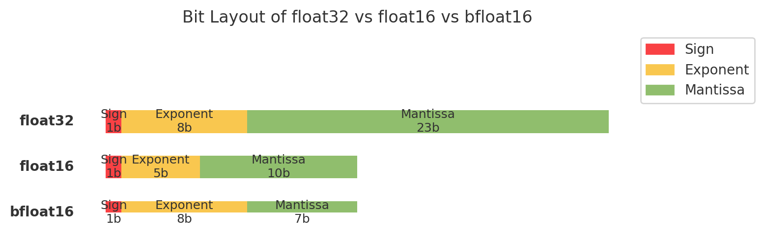
bfloat16 , developed by Google Brain, is especially notable because it retains the full 8-bit exponent of float32 , offering a wide dynamic range. While its 7-bit mantissa provides less precision, this makes it more numerically stable than float16 , particularly for training deep networks
Integer Quantization
Integer quantization maps real-valued numbers to a discrete integer range using an affine transformation. This process enables efficient inference using low-precision arithmetic.
Quantization: $q = \text{round}\left(\frac{x}{s}\right) + z$
Dequantization: $x \approx s \cdot (q - z)$
Where:
xis the original floatqis the quantized integersis the scale (a float)zis the zero-point (an int)
These mappings let the model operate primarily with integers during inference, reducing memory usage and enabling faster execution on integer-optimized hardware.
How Are Scale and Zero-Point Determined? (Calibration)
The scale and zero-point are calculated based on the distribution of float values in a tensor. Typically:
-
Scale (
s) is derived from the min and max float values of the tensor, and the min and max values of the quantized range (0-255 foruint8or -128 to 127 forint8)s = (x_max - x_min) / (q_max - q_min) -
Zero-point (
z) ensures that 0 is exactly representable:z = round(q_min - x_min / s)
This process of determining the appropriate scale and zero-point by observing real-valued data flowing through the model is known as calibration. It is especially important for static quantization, where activation ranges are fixed based on representative input data.
These parameters are then stored along with each quantized tensor. There are two main approaches:
- Per-tensor quantization: One scale and zero-point for the entire tensor.
- Per-channel quantization: Separate scale and zero-point per output channel (commonly used for weights in convolutional layers).
During inference, these values are used to convert between quantized and real representations efficiently. Some characteristics:
- Aggressive memory/computation savings.
- May introduce more quantization error.
- Commonly used in edge-optimized frameworks like TensorFlow Lite and PyTorch Mobile.
Tradeoffs
Quantization enables efficient inference but can degrade accuracy, especially if done post training without calibration. To minimize this, modern techniques like Quantization Aware Training (QAT) are used, see below.
When Is Quantization Applied?
Quantization can be applied at different stages in the model lifecycle. The two primary approaches are Post Training Quantization (PTQ) and Quantization Aware Training (QAT), each with its own benefits and tradeoffs.
Post Training Quantization (PTQ)
PTQ is applied to a fully trained model without requiring any retraining. It’s simple and quick to implement, but may cause some degradation in model accuracy, especially when using aggressive quantization like int8.
Advantages:
- Easy to integrate into existing workflows
- No need to modify training code
- Can dramatically reduce model size and inference cost
Limitations:
- Accuracy may drop, especially for sensitive models or tasks
- Works best on models that are already robust to small numeric changes
Variants:
-
Dynamic Quantization:
- When? After training.
- What? Only weights are quantized and stored in
int8. Activations remain in float and are quantized dynamically during inference. - How? No calibration needed. Activation ranges are computed on-the-fly at runtime.
- Pros: Easy to apply; works well for models with large
nn.Linearlayers (e.g., NLP). - Cons: Some operations still use float intermediates; less efficient than static quantization.
-
Static Quantization:
- When? After training.
- What? Both weights and activations are quantized to
int8. - How? Requires calibration, passing representative data through the model to collect activation stats.
- Pros: Enables full integer inference; maximizes performance.
- Cons: Slightly more setup due to calibration requirement.
-
Weight-only Quantization:
- When? After training.
- What? Only weights are quantized; activations remain
float32. - How? No activation quantization, so no calibration needed.
- Pros: Reduces model size.
- Cons: Limited inference speedup since activations are still float. Only weights are quantized; activations remain in float. Saves memory, but yields limited inference speedup.
Quantization Aware Training (QAT)
QAT introduces quantization effects during the training process by simulating them using fake quantization operations. These operations emulate the behavior of quantization during the forward pass (e.g., rounding, clamping) while still allowing gradients to flow through in full precision during the backward pass. This enables the model to learn to be robust to quantization effects while maintaining effective training dynamics.
Advantages:
- Highest accuracy among quantized models
- Especially useful for smaller or sensitive models that suffer from PTQ degradation
Limitations:
- Requires retraining or fine-tuning
- Slightly slower training due to added quantization simulation steps
QAT is particularly effective for compact architectures like MobileNet or for models deployed on edge devices where low-precision inference is essential and even small drops in accuracy can be problematic. (like MobileNet) or models deployed in latency-sensitive, low-precision environments (e.g., mobile or embedded devices).
Code Walkthrough
In this section I will provide a complete example of applying both Post Training Quantization (PTQ) and Quantization Aware Training (QAT) to a ResNet18 model adjusted for CIFAR-10 dataset. The code was tested to work on PyTorch 2.4 through 2.8 (nightly build) using both X86 Quantizer for CPU deployments and XNNPACK Quantizer used for mobile and edge devices. You can find the full self-contained jupyter notebooks below, or in the Neural Network Optimization GitHub repository.
- Quantization - PTQ using PyTorch 2 Export Quantization and X86 Backend
- Quantization - QAT using PyTorch 2 Export Quantization and X86 Backend
- Quantization - PTQ using PyTorch 2 Export Quantization and XNNPACK Quantizer
- Quantization - QAT using PyTorch 2 Export Quantization and XNNPACK Quantizer
Below I will go over the code for PTQ and QAT for the X86 scenario, as the edge device case is very similar.
Shared code
We start with defining some code to get the CIFAR-10 dataset, adjust the ResNet18 model, and define training and evaluation functions to measure the model’s size, accuracy, and latency. We end this section with the training and evaluation of the baseline model, before quantization.
Basic Setup
import os
import time
import warnings
from packaging import version
import numpy as np
import torch
import torch.nn as nn
from torchvision import datasets, transforms, models
from torch.quantization import quantize_dynamic
from torch.ao.quantization import get_default_qconfig, QConfigMapping
from torch.ao.quantization.quantize_fx import prepare_fx, convert_fx
from torch.utils.data import DataLoader, Subset

# ignores irrelevant warning, see: https://github.com/pytorch/pytorch/issues/149829
warnings.filterwarnings("ignore", message=".*TF32 acceleration on top of oneDNN is available for Intel GPUs. The current Torch version does not have Intel GPU Support.*")

# ignores irrelevant warning, see: https://github.com/tensorflow/tensorflow/issues/77293
warnings.filterwarnings("ignore", message=".*erase_node(.*) on an already erased node.*")

print(f"PyTorch Version: {torch.__version__}")
device = torch.device("cuda" if torch.cuda.is_available() else "cpu")
print(f"Device used: {device.type}")

skip_cpu = False # change to True to skip the slow checks on CPU
print(f"Should skip CPU evaluations: {skip_cpu}")
Get CIFAR-10 train and test sets
transform = transforms.Compose([
    transforms.Resize(32),
    transforms.ToTensor(),
    transforms.Normalize((0.5,), (0.5,))
])

train_dataset = datasets.CIFAR10(root="./data", train=True, download=True, transform=transform)
train_loader = DataLoader(
    datasets.CIFAR10(root="./data", train=True, download=True, transform=transform),
    batch_size=128, shuffle=True
)

test_dataset = datasets.CIFAR10(root="./data", train=False, download=True, transform=transform)
test_loader = DataLoader(
    datasets.CIFAR10(root="./data", train=False, download=True, transform=transform),
    batch_size=128,
    shuffle=False,
    num_workers=2,
    drop_last=True,
)

calibration_dataset = Subset(train_dataset, range(256))
calibration_loader = DataLoader(calibration_dataset, batch_size=128, shuffle=False)
Adjust ResNet18 network for CIFAR-10 dataset
def get_resnet18_for_cifar10():
    """
    Returns a ResNet-18 model adjusted for CIFAR-10:
    - 3x3 conv with stride 1
    - No max pooling
    - 10 output classes
    """
    model = models.resnet18(weights=None, num_classes=10)
    model.conv1 = nn.Conv2d(3, 64, kernel_size=3, stride=1, padding=1, bias=False)
    model.maxpool = nn.Identity()
    return model.to(device)

model_to_quantize = get_resnet18_for_cifar10()
Define Train and Evaluate functions
def train(model, loader, epochs, lr=0.01, save_path="model.pth", silent=False):
    """
    Trains a model with SGD and cross-entropy loss.
    Loads from save_path if it exists.
    """

    try:
        model.train()
    except NotImplementedError:
        torch.ao.quantization.move_exported_model_to_train(model)

    if os.path.exists(save_path):
        if not silent:
            print(f"Model already trained. Loading from {save_path}")
        model.load_state_dict(torch.load(save_path))
        return

    # no saved model found. training from given model state

    criterion = nn.CrossEntropyLoss()
    optimizer = torch.optim.SGD(model.parameters(), lr=lr, momentum=0.9)

    for epoch in range(epochs):
        for x, y in loader:
            x, y = x.to(device), y.to(device)
            optimizer.zero_grad()
            loss = criterion(model(x), y)
            loss.backward()
            optimizer.step()
        if not silent:
            print(f"Epoch {epoch+1}: loss={loss.item():.4f}")
            evaluate(model, f"Epoch {epoch+1}")
            try:
                model.train()
            except NotImplementedError:
                torch.ao.quantization.move_exported_model_to_train(model)

    if save_path:
        torch.save(model.state_dict(), save_path)
        if not silent:
            print(f"Training complete. Model saved to {save_path}")

def evaluate(model, tag):
    """
    Evaluates the model on test_loader and prints accuracy.
    """

    try:
        model.eval()
    except NotImplementedError:
        model = torch.ao.quantization.move_exported_model_to_eval(model)

    model.to(device)
    correct = total = 0
    with torch.no_grad():
        for x, y in test_loader:
            x, y = x.to(device), y.to(device)
            preds = model(x).argmax(1)
            correct += (preds == y).sum().item()
            total += y.size(0)
    accuracy = correct / total
    print(f"Accuracy ({tag}): {accuracy*100:.2f}%")
Define helper functions to measure latency
class Timer:
    """
    A simple timer utility for measuring elapsed time in milliseconds.

    Supports both GPU and CPU timing:
    - If CUDA is available, uses torch.cuda.Event for accurate GPU timing.
    - Otherwise, falls back to wall-clock CPU timing via time.time().

    Methods:
        start(): Start the timer.
        stop(): Stop the timer and return the elapsed time in milliseconds.
    """

    def __init__(self):
        self.use_cuda = torch.cuda.is_available()
        if self.use_cuda:
            self.starter = torch.cuda.Event(enable_timing=True)
            self.ender = torch.cuda.Event(enable_timing=True)

    def start(self):
        if self.use_cuda:
            self.starter.record()
        else:
            self.start_time = time.time()

    def stop(self):
        if self.use_cuda:
            self.ender.record()
            torch.cuda.synchronize()
            return self.starter.elapsed_time(self.ender)  # ms
        else:
            return (time.time() - self.start_time) * 1000  # ms

def estimate_latency(model, example_inputs, repetitions=50):
    """
    Returns avg and std inference latency (ms) over given runs.
    """

    timer = Timer()
    timings = np.zeros((repetitions, 1))

    # warm-up
    for _ in range(5):
        _ = model(example_inputs)

    with torch.no_grad():
        for rep in range(repetitions):
            timer.start()
            _ = model(example_inputs)
            elapsed = timer.stop()
            timings[rep] = elapsed

    return np.mean(timings), np.std(timings)

def estimate_latency_full(model, tag, skip_cpu):
    """
    Prints model latency on GPU and (optionally) CPU.
    """

    # estimate latency on CPU
    if not skip_cpu:
        example_input = torch.rand(128, 3, 32, 32).cpu()
        model.cpu()
        latency_mu, latency_std = estimate_latency(model, example_input)
        print(f"Latency ({tag}, on CPU): {latency_mu:.2f} ± {latency_std:.2f} ms")

    # estimate latency on GPU
    example_input = torch.rand(128, 3, 32, 32).cuda()
    model.cuda()
    latency_mu, latency_std = estimate_latency(model, example_input)
    print(f"Latency ({tag}, on GPU): {latency_mu:.2f} ± {latency_std:.2f} ms")

def print_size_of_model(model, tag=""):
    """
    Prints model size (MB).
    """

    torch.save(model.state_dict(), "temp.p")
    size_mb_full = os.path.getsize("temp.p") / 1e6
    print(f"Size ({tag}): {size_mb_full:.2f} MB")
    os.remove("temp.p")
Train full model
train(model_to_quantize, train_loader, epochs=15, save_path="full_model.pth")
Evaluate full model
# get full model size
print_size_of_model(model_to_quantize, "full")

# evaluate full accuracy
accuracy_full = evaluate(model_to_quantize, 'full')

# estimate full model latency
estimate_latency_full(model_to_quantize, 'full', skip_cpu)
Results:
Size (full): 44.77 MB
Accuracy (full): 80.53%
Latency (full, on CPU): 804.16 ± 57.55 ms
Latency (full, on GPU): 16.39 ± 0.30 ms
Post Training Quantization (PTQ)
The basic flow is as follow:
- Export the model to to a stable, backend-agnostic format that’s suitable for transformations, optimizations, and deployment.
- Define the quantizer that will prepare the model for quantization. Here I used the X86 for CPU deployments, but there is a simple variant that works better for mobile and edge devices working on ARM CPUs.
- Preparing the model for quantization. For example, folding batch-norm into preceding conv2d operators, and inserting observers in appropriate places to collect activation statistics needed for calibration.
- Running inference on calibration data to collect activation statistics
- Converts calibrated model to a quantized model. While the quantized model already takes less space, it is not yet optimized for the final deployment.
from torch.ao.quantization.quantize_pt2e import (
  prepare_pt2e,
  convert_pt2e,
)

import torch.ao.quantization.quantizer.x86_inductor_quantizer as xiq
from torch.ao.quantization.quantizer.x86_inductor_quantizer import X86InductorQuantizer

# batch of 128 images, each with 3 color channels and 32x32 resolution (CIFAR-10)
example_inputs = (torch.rand(128, 3, 32, 32).to(device),)

# export the model to a standardized format before quantization
if version.parse(torch.__version__) >= version.parse("2.5"): # for pytorch 2.5+
    exported_model  = torch.export.export_for_training(model_to_quantize, example_inputs).module()
else: # for pytorch 2.4
    from torch._export import capture_pre_autograd_graph
    exported_model = capture_pre_autograd_graph(model_to_quantize, example_inputs)

# quantization setup for X86 Inductor Quantizer
quantizer = X86InductorQuantizer()
quantizer.set_global(xiq.get_default_x86_inductor_quantization_config())

# preparing for PTQ by folding batch-norm into preceding conv2d operators, and inserting observers in appropriate places
prepared_model = prepare_pt2e(exported_model, quantizer)

# run inference on calibration data to collect activation stats needed for activation quantization
def calibrate(model, data_loader):
    torch.ao.quantization.move_exported_model_to_eval(model)
    with torch.no_grad():
        for image, target in data_loader:
            model(image.to(device))
calibrate(prepared_model, calibration_loader)

# converts calibrated model to a quantized model
quantized_model = convert_pt2e(prepared_model)

# export again to remove unused weights after quantization
if version.parse(torch.__version__) >= version.parse("2.5"): # for pytorch 2.5+
    quantized_model = torch.export.export_for_training(quantized_model, example_inputs).module()
else: # for pytorch 2.4
    quantized_model = capture_pre_autograd_graph(quantized_model, example_inputs)
Evaluate quantized model
# get quantized model size
print_size_of_model(quantized_model, "quantized")

# evaluate quantized accuracy
accuracy_full = evaluate(quantized_model, 'quantized')

# estimate quantized model latency
estimate_latency_full(quantized_model, 'quantized', skip_cpu)
Results:
Size (quantized): 11.26 MB
Accuracy (quantized): 80.45%
Latency (quantized, on CPU): 1982.11 ± 229.35 ms
Latency (quantized, on GPU): 37.15 ± 0.08 ms
Notice the space dropped by 75%, but CPU and GPU latency more than doubled. This is because the model while quantized is not optimized yet to run on the specific device. This will happen in the next section.
Optimize quantized model for inference
Here we do the final optimization to squeeze the performance. This uses C++ wrapper which reduces the Python overhead
# enable the use of the C++ wrapper for TorchInductor which reduces Python overhead
import torch._inductor.config as config
config.cpp_wrapper = True

# compiles quantized model to generate optimized model
with torch.no_grad():
    optimized_model = torch.compile(quantized_model)
Evaluate optimized model
# get optimized model size
print_size_of_model(optimized_model, "optimized")

# evaluate optimized accuracy
accuracy_full = evaluate(optimized_model, 'optimized')

# estimate optimized model latency
estimate_latency_full(optimized_model, 'optimized', skip_cpu)
Results:
Size (optimized): 11.26 MB
Accuracy (optimized): 79.53%
Latency (optimized, on CPU): 782.53 ± 51.36 ms
Latency (optimized, on GPU): 13.80 ± 0.28 ms
Notably, it achieves a 75% reduction in space, reduces GPU latency by 16% and 3% on CPU, with only a 1% drop in accuracy.
Quantization Aware Training (QAT)
In QAT the basic flow is very similiar to PTQ, the main difference is the replacement of the calibration step that collects activation statistics with a much longer fine-tuning step which fine-tunes the model considering the quantization constraints. The collection of activation statistics also happens, as part of the fine-tuning process.
from torch.ao.quantization.quantize_pt2e import (
  prepare_qat_pt2e,
  convert_pt2e,
)

import torch.ao.quantization.quantizer.x86_inductor_quantizer as xiq
from torch.ao.quantization.quantizer.x86_inductor_quantizer import X86InductorQuantizer

# batch of 128 images, each with 3 color channels and 32x32 resolution (CIFAR-10)
example_inputs = (torch.rand(128, 3, 32, 32).to(device),)

# export the model to a standardized format before quantization
if version.parse(torch.__version__) >= version.parse("2.5"): # for pytorch 2.5+
    exported_model  = torch.export.export_for_training(model_to_quantize, example_inputs).module()
else: # for pytorch 2.4
    from torch._export import capture_pre_autograd_graph
    exported_model = capture_pre_autograd_graph(model_to_quantize, example_inputs)

# quantization setup for X86 Inductor Quantizer
quantizer = X86InductorQuantizer()
quantizer.set_global(xiq.get_default_x86_inductor_quantization_config())

# inserts fake quantizes in appropriate places in the model and performs the fusions, like conv2d + batch-norm
prepared_model = prepare_qat_pt2e(exported_model, quantizer)

# fine-tune with quantization constraints
train(prepared_model, train_loader, epochs=3, save_path="qat_model_x86.pth")

# converts calibrated model to a quantized model
quantized_model = convert_pt2e(prepared_model)

# export again to remove unused weights after quantization
if version.parse(torch.__version__) >= version.parse("2.5"): # for pytorch 2.5+
    quantized_model = torch.export.export_for_training(quantized_model, example_inputs).module()
else: # for pytorch 2.4
    quantized_model = capture_pre_autograd_graph(quantized_model, example_inputs)
Evaluate quantized model
# get quantized model size
print_size_of_model(quantized_model, "quantized")

# evaluate quantized accuracy
accuracy_full = evaluate(quantized_model, 'quantized')

# estimate quantized model latency
estimate_latency_full(quantized_model, 'quantized', skip_cpu)
Results:
Size (quantized): 11.26 MB
Accuracy (quantized): 80.57%
Latency (quantized, on CPU): 1617.82 ± 158.67 ms
Latency (quantized, on GPU): 33.62 ± 0.16 ms
Optimize quantized model for inference
# enable the use of the C++ wrapper for TorchInductor which reduces Python overhead
import torch._inductor.config as config
config.cpp_wrapper = True

# compiles quantized model to generate optimized model
with torch.no_grad():
    optimized_model = torch.compile(quantized_model)
Evaluate optimized model
# get optimized model size
print_size_of_model(optimized_model, "optimized")

# evaluate optimized accuracy
accuracy_full = evaluate(optimized_model, 'optimized')

# estimate optimized model latency
estimate_latency_full(optimized_model, 'optimized', skip_cpu)
Results:
Size (optimized): 11.26 MB
Accuracy (optimized): 79.54%
Latency (optimized, on CPU): 831.76 ± 39.63 ms
Latency (optimized, on GPU): 13.71 ± 0.24 ms
While in this small-scale model the results of QAT are very similar to PTQ, it is suggested that for larger models QAT has an opportunity to provide higher accuracy than the PTQ variant.
Comparison of PTQ and QAT Results
Below is a summary table comparing the baseline model with the Post Training Quantization (PTQ) and Quantization Aware Training (QAT) results based on our CIFAR-10 ResNet18 experiments:
| Method | Model Size | Accuracy | GPU Latency (ms) | CPU Latency (ms) |
|---|---|---|---|---|
| Baseline (no quantization) | 44.77 MB | 80.53% | 16.39 ± 0.30 ms | 804.16 ± 57.55 ms |
| Post Training Quantization | 11.26 MB | 79.53% | 13.80 ± 0.28 ms | 782.53 ± 51.36 ms |
| Quantization Aware Training | 11.26 MB | 79.54% | 13.71 ± 0.24 ms | 831.76 ± 39.63 ms |
Summary
Quantization is a powerful technique for compressing and accelerating deep learning models by lowering numerical precision. PyTorch provides flexible APIs for applying both Post Training Quantization (PTQ) and Quantization Aware Training (QAT).
- Use PTQ when simplicity and speed are key, and you can tolerate some loss in accuracy.
- Use QAT when you need the best possible performance from quantized models, especially for smaller or sensitive models.
With good calibration and training strategies, quantization can reduce model size and inference time significantly with minimal impact on performance.
References
For additional details, the following sources were helpful when preparing this post.
- PyTorch Documentation: Quantization
- PyTorch Documentation: PyTorch 2 Export Post Training Quantization
- PyTorch Documentation: PyTorch 2 Export Quantization-Aware Training (QAT)
- PyTorch Documentation: PyTorch 2 Export Quantization with X86 Backend through Inductor
- PyTorch Dev Discussions: TorchInductor Update 6: CPU backend performance update and new features in PyTorch 2.1